Analysing a Simulated Signal
Overview
Simple-pe identifies the observable features in the gravitational-wave signal and uses them to perform parameter estimation. In particular, the analysis identifies the peak of the SNR across the mass and aligned spin space. It then uses a quadratic approximation to generate posterior distributions for those parameters. Full posteriors for masses, spins, distance and orientation are generated using this information and also the measured SNR in additional waveform features: the second GW polarization, higher order multipoles and precession harmonics. Details are given in Simple parameter estimation using observable features of gravitational-wave signals.
Example: Simulated signal
In this example, we analyze a simulated signal, embedded in zero noise, in
data from the LIGO and Virgo observatories. The analysis is run using the
simple-pe-pipe executable.
The configuration is specified using the configration file
 1[pesummary]
 2channels={H1:INJ, L1:INJ, V1:INJ}
 3injection=injection_params.json
 4truth=injection_params.json
 5outdir=outdir
 6accounting_group=UNKNOWN
 7accounting_group_user=albert.einstein
 8f_low=20
 9f_high=2048
10trigger_parameters=trigger_parameters.json
11approximant=IMRPhenomXPHM
12asd={H1:aligo_O4high.txt,L1:aligo_O4high.txt,V1:avirgo_O4high_NEW.txt}
13generate_corner=True
which can be launched with:
simple_pe_pipe config.ini
For this example, the simulated parameters are specified in the file
injection_params.json which are used to generate the signal. The
trigger_parameters file contains the starting parameters for the
optimization of the SNR and the truth file contains the actual values
— these are only used to plot the actual parameter values on the final
result plots. The network is specified by the asd dictionary with
instrument sensitivities.
Note
The auxiliary data can be downloaded from here.
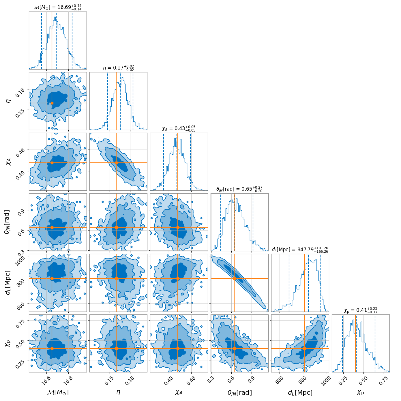
Below is a corner plot showing the obtained posterior distribution when
using the IMRPhenomXPHM waveform model (Phys.Rev.D 103 (2021) 10,
104056):

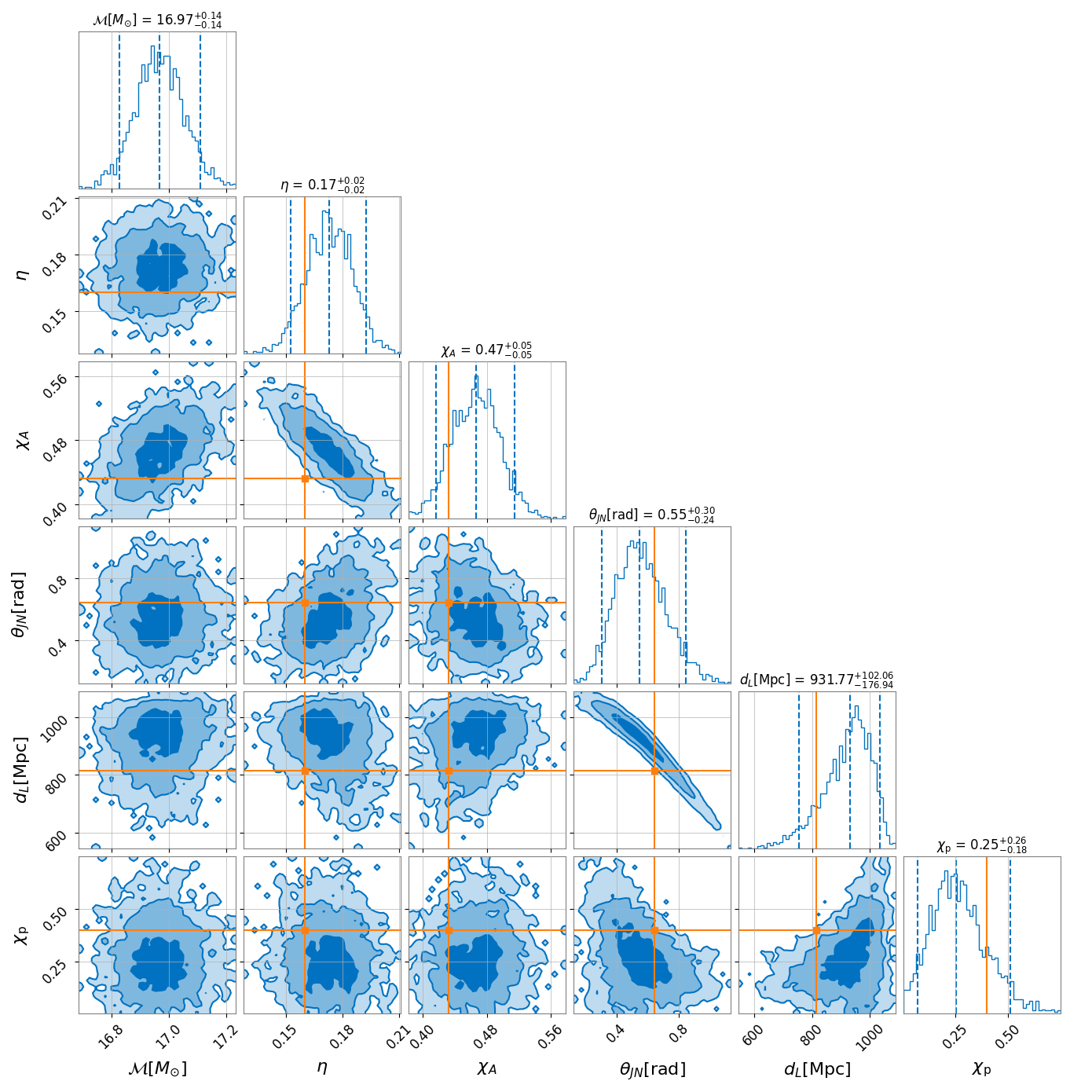
and below is a corner plot showing the obtained posterior distribution when
using the IMRPhenomTPHM waveform model (Phys.Rev.D 105 (2022) 8,
084040):

Both of these analyses were performed as part of simple-pe’s
continuous integration and are therefore using the latest version of the code.